Timsort

Most programmers would be familiar with some fundamental sorting algorithms such as bubble sort, selection sort, insertion sort, and merge sort. Then which algorithm does Python’s built-in sort() use to sort arrays? It’s Timsort. What’s more noteworthy is that Timsort has also been adopted by Android platform, V8(JS engine), Swift and Rust. Why? It’s practical.

In this post, I’m going to summarize Timsort. But before getting into it, I’ll give a brief overview of insertion sort and merge sort as both algorithms are leveraged by Timsort. Any readers well acquainted with these algorithms can skip these parts and head over to Timsort right away.

Time Complexities

	Worst-case	Best-case	Average
Insertion Sort	O(n^2)	Ω(n)	O(n^2)
Merge Sort	O(n log n)	Ω(n log n)	O(n log n)
Timsort	O(n log n)	Ω(n)	O(n log n)

Insertion Sort

Insertion sort builds the sorted array in place, shifting elements out of the way if necessary to make room. The easiest way to remind of insertion sort is thinking of sorting playing cards. You’d normally pick up a card, compare it with the rest, find the correct position, insert the card, and repeat until all cards are sorted. Unlike bubble sort and selection sort, insertion sort doesn’t have to go through an array multiple times, instead, it only needs to move forward through the array once.

Here’s the pseudocode:

Call the first element of the array "sorted."
Repeat until all elements are sorted:
    Look at the next unsorted element
    Insert into the "sorted" portion by shifting the requisite number of elements

The visual explanation is as follows:

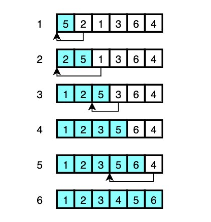
1. The first element 5 is declared as ‘sorted’. And in order to put the next unsorted element 2 in front of 5, 5 is moved to where 2 was and 2 is put where 5 was in memory. (shifted)
2. To insert the next unsorted element 1 to the correct position, 2 and 5 have to be moved over to make room for 1. Then 1 goes in to where 2 was.
3. This time, only 5 has to be moved over to get 3 into the correct position.
4. As 6 is larger than every element in the already sorted array, nothing is shifted and 6 is delcared a ‘sorted’.
5. Again, 5 and 6 are moved to make room for 4, and 4 is moved to where 5 was.
6. Everything is sorted.

Considerting that every shift costs:

• Worst-case scenario: The array is in reverse order.
• Best-case scenario: The array is already sorted. (No shift is required)

Binary Insertion Sort

In the example above, I only explained the shifting and skipped how to find the proper location to insert the selected element at each iteration. With linear search which is the basic method of insertion sort, it takes O(n). But this can be reduced to O(n log n) by using binary search. This is binary insertion sort.

Merge Sort

The idea is to sort smaller arrays and then merge those arrays together in sorted order, which is called divide-and-conquer. And it does does this by doing recursion. As a side note, recursion takes up more memory to use call stack.

Here’s the pseudocode:

Sort the left half of the array (assuming n > 1)
Sort the right half of the array (assuming n > 1)
Merge the two halves together

The visual explanation is as follows:

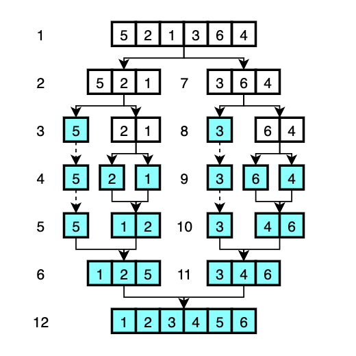
1. The array is divided into two arrays - [5, 2, 1] and [3, 6, 4].
2. The left half of the array [5, 2, 1] is to be sorted. This again divided into two arrays - [5] and [2, 1].
3. [5] is declared as ‘sorted’ as it only has one element. The next array to sort is the right half of the array [2, 1].
4. [2, 1] is divided again. The left array [2] is declared as ‘sorted’ and the right array [1] is also declard as ‘sorted’.
5. Compare the first element of the left array which is 2 and the first element of the right array which is 1. Figure out which one is smaller. The smaller element 1 becomes the first element of the new sorted array. And 2 becomes the second element of the new array.
6. Just like step 5, compare the first element of the left array which is 5 and the first element of the right array which 1. Figure out which one is smaller. The smaller element 1 from the right array becomes the first element of the new sorted array. The next decision is to compare 5 and 2, so 2 becomes the second element of the new array. The last element 5 becomes the third element of the new array. Now we have the sorted array of [1, 2, 5].
7. (Repeat the step 2 with different elements.)
8. (Repeat the step 3 with different elements.)
9. (Repeat the step 4 with different elements.)
10. (Repeat the step 5 with different elements.)
11. (Repeat the step 6 with different elements.)
12. Now that we have sorted the left half and the right half of the original array, merge two halves into one. This is done by going through the same process that we did for merging.

With merge sort, even if the array is already sorted, we still have to recursively divide and conquer. So the time complexity of best-case and worst-case is just O(n log n). Therefore, merge sort can be a better solution for sorting arrays that would be the worst-case scenario in insertion sort.

In-place Merge Sort

The standard implementation of merge sort requires the memory space of the input size. In-place merge sorts are variants to attempt to reduce this memory requirement by sorting a list in place, and there are several implementations. The space complexity of any in-place merge sort would still be O(n) just like standard merge sort, however, remember that asymptotic complexity does not necessarily mean practical complexity.

Timsort

Timsort is a hybrid stable sorting algorithm based on insertion sort and merge sort. It takes advantage of already sorted elements that exist in most real-world data and implements several optimization techniques in order to minimize the total number of comparisons and memory usage. In other words, the detailed implementation is quite sophisticated.

In a nutshell, Timsort does two things concurrently:

1. Creating runs until all data is traversed.
2. Merging runs until only one run remains.

(And yes, I oversimplified it. And yet, I did it.)

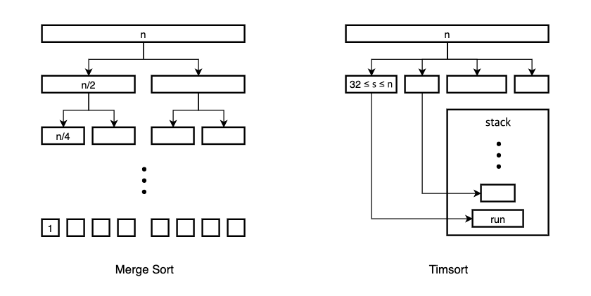
Creating Runs

While merge sort divides the array into the smallest unit that is 1 element, Timsort ensures that every sublist is longer than the minimum run size - minrun. Minrun is chosen from the range 32 to 64 at the beginning of the algorithm. The goal of minrun is to optimize the algorithm because merging is most efficient when the size of the run is of power of two. The sublists are called runs. When creating runs, Timsort uses binary insertion sort until the minrun is reached. Therefore, runs are sorted lists. These runs are put into a stack.

Natural Runs

Timsort takes advantage of already sorted elements that exist in most real-world data. These are called natural runs. Therefore, any set of consecutive ordered elements in a dataset is considered a natural run. If a run reaches the minrun and the next elements to sort are all already sorted, they are continually inserted into this run. This is what makes Timsort to achieve Ω(n) even if the input size is larger than minrun.

Merging Runs

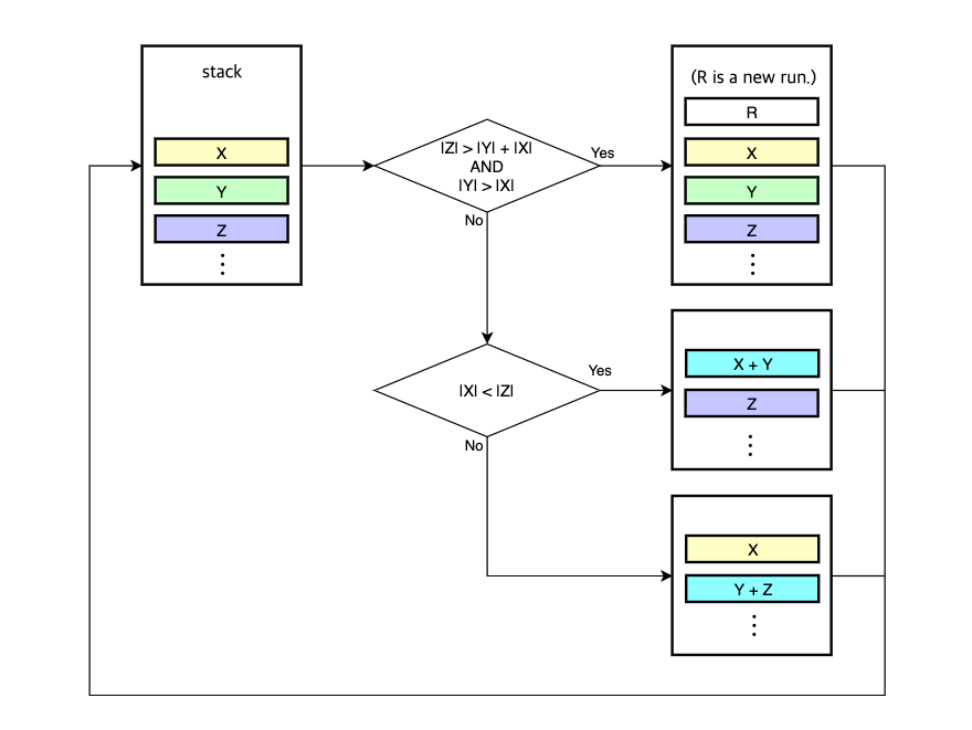
Merging happens whenever the three runs on the top of the stack, X, Y, Z violate any of these two invariants:

1. |Z| > |Y| + |X|
2. |Y| > |X|

If any invariant is violated, Y is merged with the smaller of X or Z. If there’s no violation, a new run is searched. The goal of this process is to achieve balanced merges where the sizes of the two runs are similar to one another.

Here’s an example. Consider the three runs on the top of the stack, the sizes of each run are as follows:

• |X|: 40
• |Y|: 32
• |Z|: 80

In this example, X is larger than Y and it violates one of the invariants that is |Y| > |X|. Therefore, Y must be merged with X or Z. In this case, X is the one that is merged with Y because X is smaller than Z. After the merge, the sizes of the two runs on the top of the stack are as follows:

• |X|: 72
• |Y|: 80

I drew a following diagram for easier understanding:

In-place Merging

To reduce the both time and space overhead, Timsort supports in-place merging. Unlike merge sort where the temporary buffer must be allocated with the same size of the input, Timsort requires only the smaller size of two runs at most.

This may be best understood with an example:

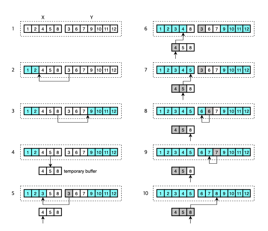
1. Here are two runs to merge. X is the first run and Y is the second.
2. Timsort first uses binary search to find the correct location for the first element of Y that is 3 to be inserted in X. The smaller elements of this location [1, 2] are already in their place and don’t need to be merged.
3. Again, do binary search to find the correct location for the last element of X that is 8 to be inserted in Y. The larger elements of this location [9, 10, 11, 12] are already in their place and don’t need to be merged.
4. Now that the only elements to be moved are [4, 5, 8] and [3, 6, 7], the smaller of the two is copied into temporary buffer. In this example, both sizes are the same so the first one is copied.
5. The elements in the temporary memory are to be merged with the larger run Y. So, the first element 4 is compared with 3 and the smaller is merged into the combined space of the two runs. 3 is now sorted.
6. The smaller of 4 and 6 is merged. 4 is now sorted.
7. The smaller of 5 and 6 is merged. 5 is now sorted.
8. The smaller of 8 and 6 is merged. 6 is now sorted.
9. The smaller of 8 and 7 is merged. 7 is now sorted.
10. The only remaining element 8 is finally sorted and the merge is done.

Note that only a temporary memory whose size is of the smaller of the remaining elements of the two runs is allocated.

And merging can be done in the opposite direction to the example here. Descending runs are later reversed and then put into the stack.

The example here is simplified and the runs are small. However, the real world data, or more specifically, the real world runs are surely much larger and it is highly likely that more consecutive elements are still in one of two runs, thus comparing in a linear fashion wouldn’t be the best way in those cases. This is where galloping mode comes in.

Galloping Mode

Galloping mode is another optimization technique to reduce the number of comparisons when finding a correct location for an element. In galloping mode, assuming that X is the shorter run, it searches Y for where X[0] belongs by performing exponential search, also known as galloping search. It first compares X[0] with Y[0] and then Y[1], Y[3], Y[7], …, Y[2**i - 1], …, until finding the k such that Y[2**(k-1)] <= X[0] < Y[2**k]. After this stage, Timsort switches to binary search to find X[0] in the last range found from galloping search. Then, when is this galloping mode triggered? It’s when min_gallop is reached. More on this in a moment.

Here’s an example. Two runs, X and Y, are in the middle of merging and it’s time to find 20 in Y.

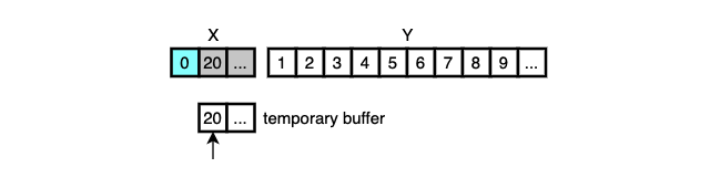
Galloping mode is not used at the beginning of merging. So 20 is compared with Y[0] and the smaller is moved into the final array. This goes on with Y[1], Y[2], Y[3], …, all the way up until it finds the proper location for X[0] or the number of consecutive elements selected from Y reaches 7, which is the initial value of min_gallop. It’s called One-pair-at-a-time mode.

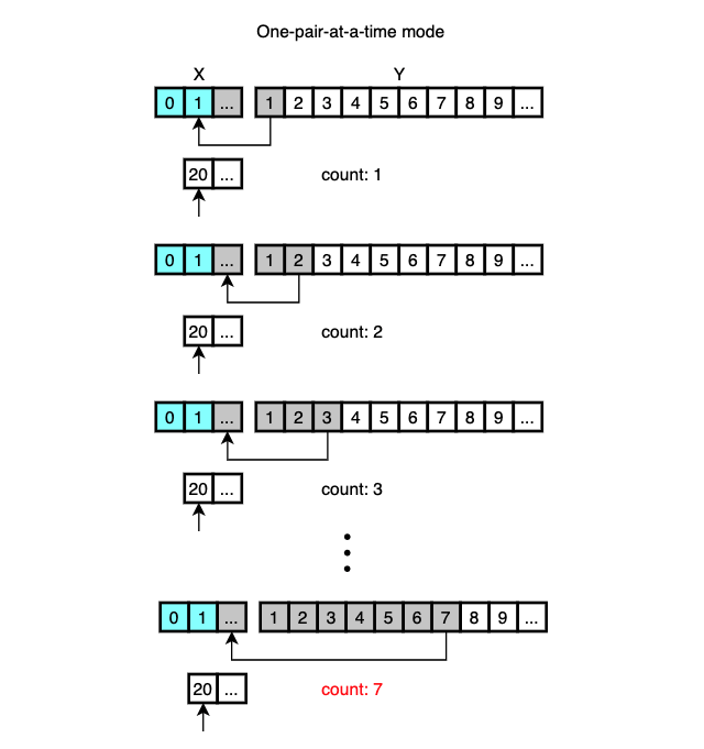
When the number of consecutively selected elements reaches 7, considering that the runs are real-worl data, it’s sensible to assume that many more consecutive elements in Y may still be smaller than X[0] so jumping some elements may help to reduce unnecessary comparisons and the smaller elements can be moved in one chunk. This is done via galloping search and binary search. With these two search algorithms, every search takes at most 2*log(Y) comparisons.

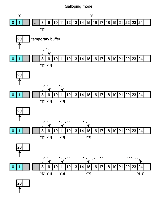
After galloping search finds the range where X[0] belongs to, binary search is performed to find the exact location in that range. The selected elements are then moved to the final array in a chunk.

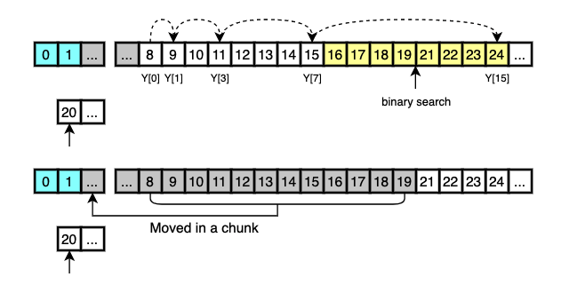
What happens next is that 20 is moved to the final array and 21 is searched in X.

The galloping mode is used until the number of consecutive elements copied from both runs is smaller than min_gallop. While Tim Peter, the creator of Timsort, described it as a minor improvement, min_gallop is adaptive. When the algorithm finds that galloping mode actually pays off, it calls merge_hi() to increase min_gallop by 1 so that the return to galloping mode is encouraged. Otherwise, it calls merge_lo() to decrease it by 1 to discourage galloping mode.

Note that galloping mode is not more efficient than simple one-pair-at-a-time mode when X[0] is not in the first seven elements in Y. For instance, if X[0] belongs right before Y[2], galloing mode requires a total of 4 comparisons while linear search would take 3 comparisons.

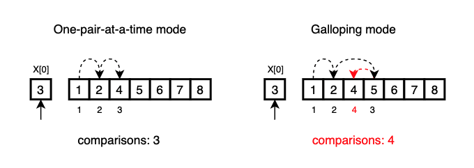
This gallop penalty can be prevented by increasing min_gallop large enough so that galloping mode is not triggered often for random data. It indicates why 7 is a good initial threshold to watch whether galloping mode pays off or not.

That’s it. Although this is pretty much a summarized version of Timsort, I hope the illustrations in this page will help you understand the concepts. For more detailed description, you may refer to this text.

Conclusion

Timsort is known to be faster than many other sorting algorithms in most cases. Moreover, if an input is already almost sorted, it takes O(n) whereas merge sort always takes O(n log n) regardless of the initial state of the input. These benefits are achieved by:

• Leveraging two fundamental algorithms; insertions sort and merge sort,
• Taking advantage of already sorted elements that exist in most real-world data,
• And implementing some optimization techniques such as minrun, in-place merging, and galloping mode.

Real-world data are real-world problems and I think Timsort is more focused on solving those real-world problems. This is why Timsort is not only fast but also practical.